Matrix calculations with Groovy, Apache Commons Math, ojAlgo, Nd4j and EJML

The Fibonacci sequence has origins in India centuries earlier but is named after the Italian author of the publication, The Book of Calculation, published in 1202. In that publication, Fibonacci proposed the sequence as a means to calculate the growth of idealized (biologically unrealistic) rabbit populations. He proposed that a newly born breeding pair of rabbits are put in a field; each breeding pair mates at the age of one month, and at the end of their second month they always produce another pair of rabbits; and rabbits never die, but continue breeding forever. Fibonacci posed the puzzle: how many pairs will there be in one year? The sequence goes like this:

We can solve this problem using matrices. If we multiply the matrix by itself n times we get 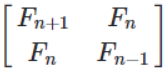. This is an operation known as matrix exponentiation. Let’s explore this problem using four of the most popular and maintained matrix libraries.

Earlier, we described the Fibonacci sequence as being for unrealistic rabbit populations, where rabbits never died and continued breeding forever. It turns out that Fibonacci matrices are a special case of a more generalised model which can model realistic rabbit populations (among other things). These are Leslie matrices. For Leslie matrices, populations are divided into classes, and we keep track of birth rates and survival rates over a particular period for each class. We store this information in a matrix in a special form. The populations for each class for the next period can be calculated from those for the current period through multiplication by the Leslie matrix.

This technique can be used for animal populations or human population calculations. A Leslie matrix can help you find out if there will be enough GenX, Millenials, and GenZ tax payers to support an aging and soon retiring baby boomer population. Sophisticated animal models might track populations for an animal and for its predators or its prey. The survival and birth rates might be adjusted based on such information. Given that only females give birth, Leslie models will often be done only in terms of the female population, with the total population extrapolated from that.

We’ll show an example for kangaroo population based on this video tutorial for Leslie matrices. It can help us find out if the kangaroo population is under threat (perhaps drought, fires or floods have impacted their feeding habitat) or if favorable conditions are leading to overpopulation.

Following that example, we divide kangaroos into 3 population classes: ages 0 to 3, 3 to 6, and 6 to 9. We are going to look at the population every three years. The 0-3 year olds birthrate (B1) is 0 since they are pre-fertile. The most fertile 3-6 year olds birthrate (B2) is 2.3. The old roos (6-9) have a birthrate (B3) of 0.4. We assume no kangaroos survive past 9 years old. 60% (S1) of the young kangaroos survive to move into the next age group. 30% (S2) of the middle-aged kangaroos survive into old age. Initially, we have 400 kangaroos in each age group.

Here is what the code looks like for this model:

This code produces the following output:

After the first round, we see many young roos but a worrying drop off in the older age groups. After the second round, only the oldest age group looks worryingly small. However, with the healthy numbers in the young generation, we can see that after 10 generations that indeed, the overall population is not at risk. In fact, overpopulation might become a problem.

An early technique to encrypt a message was the Caesar cipher. It substitutes letters in the alphabet by the letter shifted a certain amount along in the alphabet, e.g. "IBM" becomes "HAL" if shifting to the previous letter and "VMS" becomes "WNT" if shifting one letter forward in the alphabet. This kind of cipher can be broken by looking at frequency analysis of letters or pattern words.

The Hill cipher improves upon the Caesar cipher by factoring multiple letters into each letter of the encrypted text. Using matrices made it practical to look at three or more symbols at once. In general, an N-by-N matrix (the key) is multiplied by an encoding of the message in matrix form. The result is a matrix representation (encoded form) of the encrypted text. We use the inverse matrix of our key to decrypt or message.

We need to have a way to convert our text message to and from a matrix. A common scheme is to encode A as 1, B as 2, and so on. We’ll just use the ascii value for each character. We define encode and decode methods to do this:

We’ll define a 2-by-2 matrix as our key and use it to encrypt. We’ll find the inverse of our key and use that to decrypt. If we wanted to, we could use a 3-by-3 key for improved security at the cost of more processing time.

Our code looks like this:

When run, it has the following output:

This offers far more security than the Caesar cipher, however, given today’s computing availability, Hill ciphers can still eventually be broken with sufficient brute force. For this reason, Hill ciphers are seldom used on their own for encryption, but they are often used in combination with other techniques to add diffusion - strengthening the security offered by the other techniques.

Our final example looks at geometrically transforming shapes. To do this, we represent the points of the shape as vectors and multiply them using transforms represented as matrices. We need only worry about the corners, since we’ll use Swing to draw our shape, and it has a method for drawing a polygon by giving its corners.

First we’ll use Groovy’s SwingBuilder to set up our frame:

We aren’t really use much of SwingBuilder’s functionality here but if we wanted to add more functionality, SwingBuilder would make that task easier.

We will actually draw our shapes within a custom component. We’ll define a few color constants, a drawPolygon method which given a matrix of points will draw those points as a polygon. We’ll also define a vectors method to convert a list of points (the corners) into vectors, and a transform method which is a factory method for creating a transform matrix.

Here is the code:

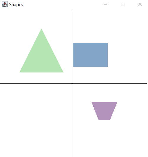
When we run this code we see our three shapes:

We can now add our transforms. We’ll have one which rotate by 90 degrees anti-clockwise. Another which enlarges a shape by 25% and one that shrinks a shape by 25%. We can combine transforms simply by multiplying them together. We’ll make two transformations of our triangle. We’ll rotate in both cases but we’ll shrink one and enlarge the other. We apply the transform simply by multiplying each point by the transform matrix. Then we’ll draw both transformed shapes as an outline rather than filled (to make it easier to distinguish the original and transformed versions). Here is the code:

For our rectangle, we’ll have one simple transform which flips the shape in the vertical axis. A second transform combines multiple changes in one transform. We could have split this into smaller transforms and the multiplied them together - but here they are all in one. We flip in the horizontal access and then apply a shear. We then draw the transformed shapes as outlines:

For our trapezoid, we create a transform which rotates 45 degrees anti-clockwise (recall sin 45° = cos 45° = 0.707). Then we create 6 transforms rotating at 45, 90, 135 and so forth. We draw each transformed shape as an outline:

When we run the entire example, here is what the output looks like:

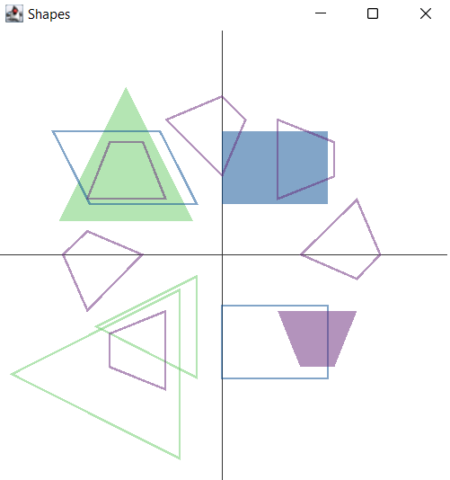
We can see here that matrix transforms give us powerful ways to manipulate images. We have used 2D images here, but the same techniques would apply to 3D shapes.

We saw earlier that some of the examples could make use of Groovy operator shorthand syntax, while others couldn’t. Here is a summary of some common methods in the libraries:

Where the library used the same name as Groovy’s method, the shorthand could be used.

Groovy offers numerous extensibility features. We won’t go into all of the details but instead refer readers to the History of Groovy paper which gives more details.

In summary, that paper defined the following extensions for Commons Math matrices:

This fixes some of the method name discrepancies in the above table. We can now use the operator shorthand for matrix and scalar addition as well as scalar multiply. We can also use the ~ (bitwiseNegate) operator when finding the inverse. The mention of double[][] during matrix construction is now also gone.

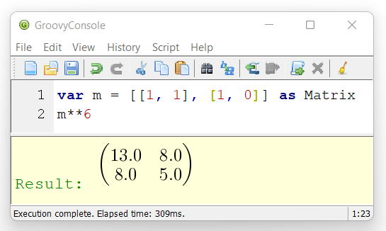
The paper goes on to discuss how to automatically add the necessary imports for a matrix library and provide aliases if needed. The imports aren’t shown for the code listings in this blog but are in the listings in the sample code repo. In any case, the imports can be "configured away" as the paper discusses. The end result is our code in its entirety can look like this:

The paper also discusses tooling extensibility, in particular the visualisation aspects of the GroovyConsole. It shows how to define an output transform which renders any matrix result using a jlatexmath library. So instead of seeing Array2DRowRealMatrix{{13.0,8.0},{8.0,5.0}}, they will see a graphical rendition of the matrix. So, the final end-user experience when using the GroovyConsole looks like this:

When using in Jupyter style environments, other pretty output styles may be supported.

We have examined a number of simple applications of matrices using the Groovy programming language and the Apache Commons Math, ojAlgo, Nd4j, and EJML libraries. You should be convinced that using matrices on the JVM isn’t hard, and you have numerous options. We also saw a brief glimpse at the Vector API which looks like an exciting addition to the JVM (hopefully arriving soon in non-preview mode).