
Natural Language Processing with Groovy™, OpenNLP, CoreNLP, Nlp4j, Datumbox, Smile, Spark NLP, DJL and TensorFlow
Published: 2022-08-07 07:34AM
Natural Language Processing is certainly a large and sometimes complex topic with many aspects. Some of those aspects deserve entire blogs in their own right. For this blog, we will briefly look at a few simple use cases illustrating where you might be able to use NLP technology in your own project.
Language Detection
Knowing what language some text represents can be a critical first step to subsequent
processing. Let’s look at how to predict the language using a pre-built model and
Apache OpenNLP. Here, ResourceHelper is a utility class used to download and cache the model. The first run may take a little while as it downloads the model. Subsequent runs should be fast. Here we are using a well-known model referenced in the OpenNLP documentation.
def helper = new ResourceHelper('https://dlcdn.apache.org/opennlp/models/langdetect/1.8.3/')
def model = new LanguageDetectorModel(helper.load('langdetect-183'))
def detector = new LanguageDetectorME(model)

[ spa: 'Bienvenido a Madrid', fra: 'Bienvenue à Paris',
  dan: 'Velkommen til København', bul: 'Добре дошли в София'
].each { k, v ->
    assert detector.predictLanguage(v).lang == k
}
The LanguageDetectorME class lets us predict the language. In general, the predictor
may not be accurate on small samples of text, but it was good enough for our example.
We’ve used the language code as the key in our map, and we check that against the
predicted language.
A more complex scenario is training your own model. Let’s look at how to do that with Datumbox. Datumbox has a pre-trained models zoo but its language detection model didn’t seem to work well for the small snippets in the next example, so we’ll train our own model. First, we’ll define our datasets:
def datasets = [
    English: getClass().classLoader.getResource("training.language.en.txt").toURI(),
    French: getClass().classLoader.getResource("training.language.fr.txt").toURI(),
    German: getClass().classLoader.getResource("training.language.de.txt").toURI(),
    Spanish: getClass().classLoader.getResource("training.language.es.txt").toURI(),
    Indonesian: getClass().classLoader.getResource("training.language.id.txt").toURI()
]
The de training dataset comes from the
Datumbox examples. The training datasets for the other
languages are from Kaggle.
We set up the training parameters needed by our algorithm:
def trainingParams = new TextClassifier.TrainingParameters(
    numericalScalerTrainingParameters: null,
    featureSelectorTrainingParametersList: [new ChisquareSelect.TrainingParameters()],
    textExtractorParameters: new NgramsExtractor.Parameters(),
    modelerTrainingParameters: new MultinomialNaiveBayes.TrainingParameters()
)
We’ll use a Naïve Bayes model with Chisquare feature selection.
Next we create our algorithm, train it with our training dataset, and then validate it against the training dataset. We’d normally want to split the data into training and testing datasets, to give us a more accurate statistic of the accuracy of our model. But for simplicity, while still illustrating the API, we’ll train and validate with our entire dataset:
def config = Configuration.configuration
def classifier = MLBuilder.create(trainingParams, config)
classifier.fit(datasets)
def metrics = classifier.validate(datasets)
println "Classifier Accuracy (using training data): $metrics.accuracy"
When run, we see the following output:
Classifier Accuracy (using training data): 0.9975609756097561
Our test dataset will consist of some hard-coded illustrative phrases. Let’s use our model to predict the language for each phrase:
[   'Bienvenido a Madrid', 'Bienvenue à Paris', 'Welcome to London',
    'Willkommen in Berlin', 'Selamat Datang di Jakarta'
].each { txt ->
    def r = classifier.predict(txt)
    def predicted = r.YPredicted
    def probability = sprintf '%4.2f', r.YPredictedProbabilities.get(predicted)
    println "Classifying: '$txt',  Predicted: $predicted,  Probability: $probability"
}
When run, it has this output:
Classifying: 'Bienvenido a Madrid',  Predicted: Spanish,  Probability: 0.83
Classifying: 'Bienvenue à Paris',  Predicted: French,  Probability: 0.71
Classifying: 'Welcome to London',  Predicted: English,  Probability: 1.00
Classifying: 'Willkommen in Berlin',  Predicted: German,  Probability: 0.84
Classifying: 'Selamat Datang di Jakarta',  Predicted: Indonesian,  Probability: 1.00
Given these phrases are very short, it is nice to get them all correct, and the probabilities all seem reasonable for this scenario.
Parts of Speech
Parts of speech (POS) analysers examine each part of a sentence (the words and potentially punctuation) in terms of the role they play in a sentence. A typical analyser will assign or annotate words with their role like identifying nouns, verbs, adjectives and so forth. This can be a key early step for tools like the voice assistants from Amazon, Apple and Google.
We’ll start by looking at a perhaps lesser known library Nlp4j before looking at some others. In fact, there are multiple Nlp4j libraries. We’ll use the one from nlp4j.org, which seems to be the most active and recently updated.
This library uses the Stanford CoreNLP library under the covers for its English POS functionality. The library has the concept of documents, and annotators that work on documents. Once annotated, we can print out all of the discovered words and their annotations:
var doc = new DefaultDocument()
doc.putAttribute('text', 'I eat sushi with chopsticks.')
var ann = new StanfordPosAnnotator()
ann.setProperty('target', 'text')
ann.annotate(doc)
println doc.keywords.collect{  k -> "${k.facet - 'word.'}(${k.str})" }.join(' ')
When run, we see the following output:
PRP(I) VBP(eat) NN(sushi) IN(with) NNS(chopsticks) .(.)
The annotations, also known as tags or facets, for this example are as follows:
PRP |
Personal pronoun |
VBP |
Present tense verb |
NN |
Noun, singular |
IN |
Preposition |
NNS |
Noun, plural |
The documentation for the libraries we are using give a more complete list of such annotations.
A nice aspect of this library is support for other languages, in particular, Japanese. The code is very similar but uses a different annotator:
doc = new DefaultDocument()
doc.putAttribute('text', '私は学校に行きました。')
ann = new KuromojiAnnotator()
ann.setProperty('target', 'text')
ann.annotate(doc)
println doc.keywords.collect{ k -> "${k.facet}(${k.str})" }.join(' ')
When run, we see the following output:
名詞(私) 助詞(は) 名詞(学校) 助詞(に) 動詞(行き) 助動詞(まし) 助動詞(た) 記号(。)
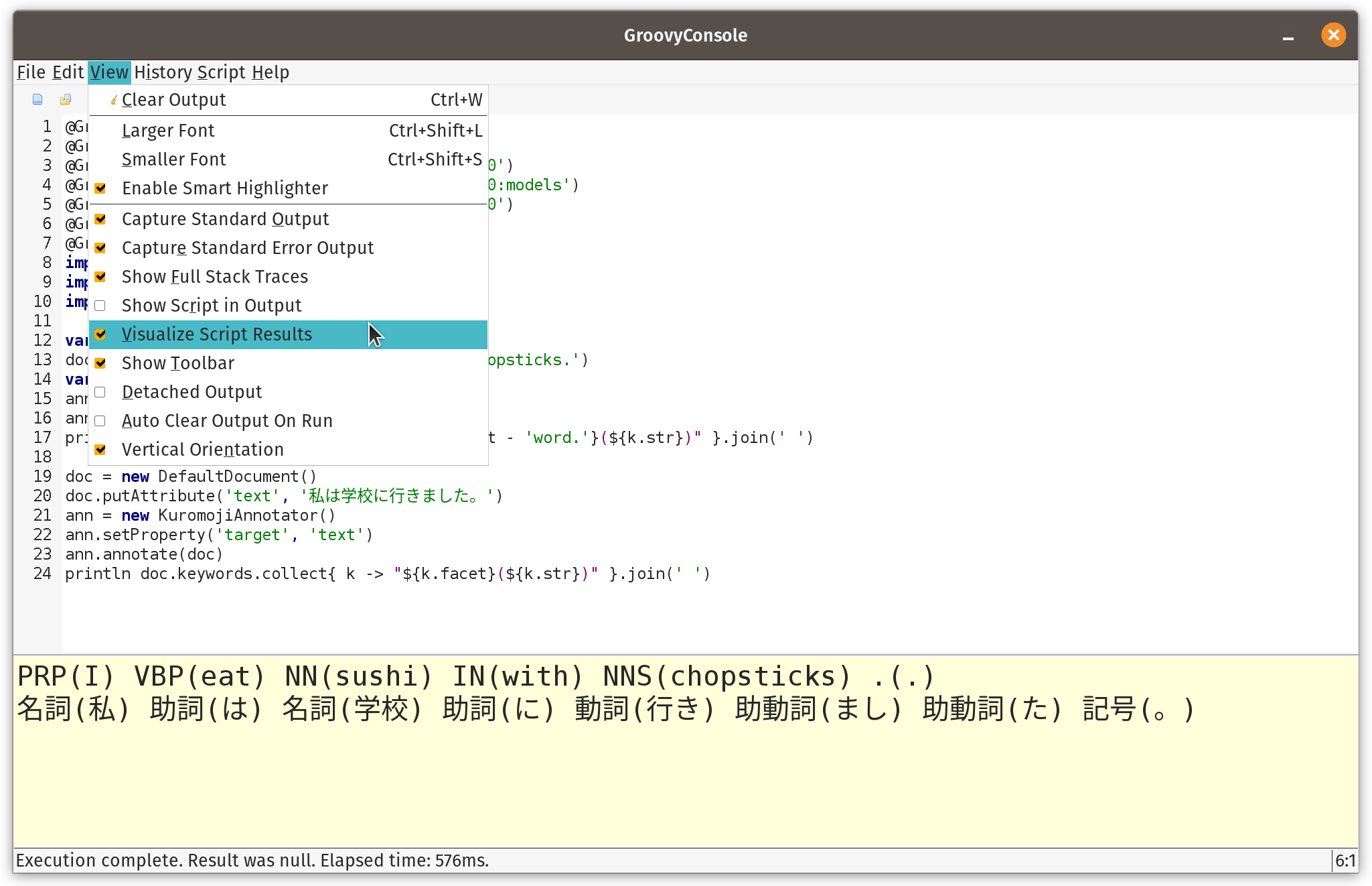
Before progressing, we’ll highlight the result visualization capabilities of the
GroovyConsole. This feature lets us write a small Groovy script which converts
results to any swing component. In our case we’ll convert lists of annotated strings
to a JLabel component containing HTML including colored annotation boxes.
The details aren’t included here but can be found in the
repo.
We need to copy that file into our ~/.groovy folder and then enable script
visualization as shown here:
Then we should see the following when running the script:
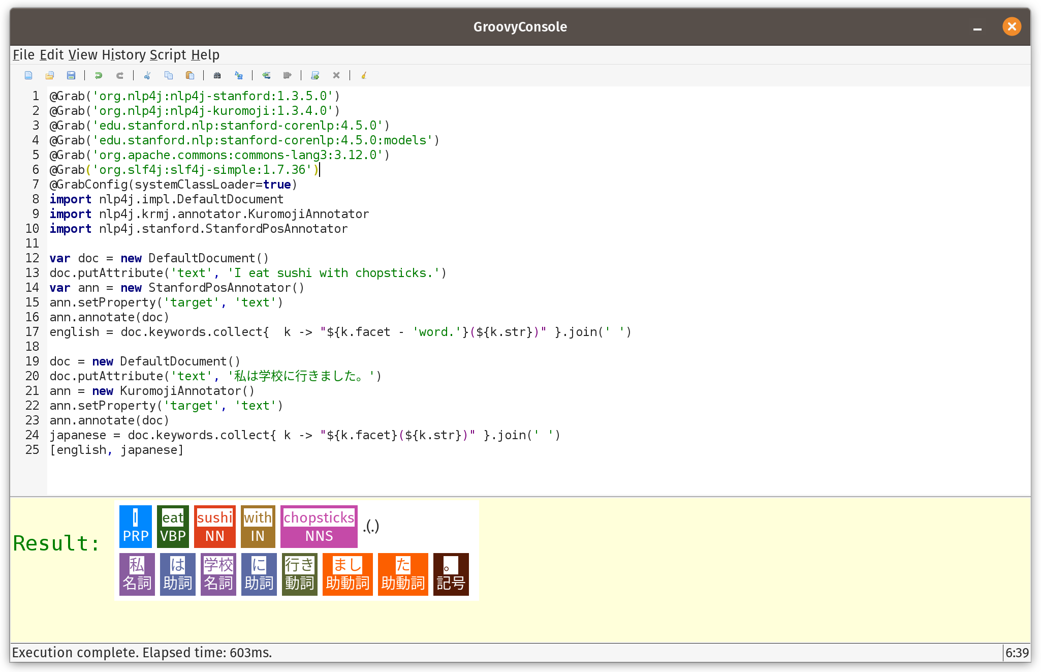
The visualization is purely optional but adds a nice touch. If using Groovy in notebook environments like Jupyter/BeakerX, there might be visualization tools in those environments too.
Let’s look at a larger example using the Smile library.
First, the sentences that we’ll examine:
def sentences = [
    'Paul has two sisters, Maree and Christine.',
    'No wise fish would go anywhere without a porpoise',
    'His bark was much worse than his bite',
    'Turn on the lights to the main bedroom',
    "Light 'em all up",
    'Make it dark downstairs'
]
A couple of those sentences might seem a little strange, but they are selected to show off quite a few of the different POS tags.
Smile has a tokenizer class which splits a sentence into words. It handles numerous cases like contractions and abbreviations ("e.g.", "'tis", "won’t"). Smile also has a POS class based on the hidden Markov model and a built-in model is used for that class. Here is our code using those classes:
def tokenizer = new SimpleTokenizer(true)
sentences.each {
    def tokens = Arrays.stream(tokenizer.split(it)).toArray(String[]::new)
    def tags = HMMPOSTagger.default.tag(tokens)*.toString()
    println tokens.indices.collect{tags[it] == tokens[it] ? tags[it] : "${tags[it]}(${tokens[it]})" }.join(' ')
}
We run the tokenizer for each sentence. Each token is then displayed directly or with its tag if it has one.
Running the script gives this visualization:
|
[Note: the scripts in the repo just print to stdout which is perfect when using the
command-line or IDEs. The visualization in the GoovyConsole kicks in only for the
actual result. So, if you are following along at home and wanting to use the
GroovyConsole, you’d change the each to collect and remove the println,
and you should be good for visualization.]
The OpenNLP code is very similar:
def tokenizer = SimpleTokenizer.INSTANCE
sentences.each {
    String[] tokens = tokenizer.tokenize(it)
    def posTagger = new POSTaggerME('en')
    String[] tags = posTagger.tag(tokens)
    println tokens.indices.collect{tags[it] == tokens[it] ? tags[it] : "${tags[it]}(${tokens[it]})" }.join(' ')
}
OpenNLP allows you to supply your own POS model but downloads a default one if none is specified.
When the script is run, it has this visualization:
|
The observant reader may have noticed some slight differences in the tags used in this library. They are essentially the same but using slightly different names. This is something to be aware of when swapping between POS libraries or models. Make sure you look up the documentation for the library/model you are using to understand the available tag types.
Entity Detection
Named entity recognition (NER), seeks to identity and classify named entities in text. Categories of interest might be persons, organizations, locations dates, etc. It is another technology used in many fields of NLP.
We’ll start with our sentences to analyse:
String[] sentences = [
    "A commit by Daniel Sun on December 6, 2020 improved Groovy 4's language integrated query.",
    "A commit by Daniel on Sun., December 6, 2020 improved Groovy 4's language integrated query.",
    'The Groovy in Action book by Dierk Koenig et. al. is a bargain at $50, or indeed any price.',
    'The conference wrapped up yesterday at 5:30 p.m. in Copenhagen, Denmark.',
    'I saw Ms. May Smith waving to June Jones.',
    'The parcel was passed from May to June.',
    'The Mona Lisa by Leonardo da Vinci has been on display in the Louvre, Paris since 1797.'
]
We’ll use some well-known models, we’ll focus on the person, money, date, time, and location models:
def base = 'http://opennlp.sourceforge.net/models-1.5'
def modelNames = ['person', 'money', 'date', 'time', 'location']
def finders = modelNames.collect { model ->
    new NameFinderME(DownloadUtil.downloadModel(new URL("$base/en-ner-${model}.bin"), TokenNameFinderModel))
}
We’ll now tokenize our sentences:
def tokenizer = SimpleTokenizer.INSTANCE
sentences.each { sentence ->
    String[] tokens = tokenizer.tokenize(sentence)
    Span[] tokenSpans = tokenizer.tokenizePos(sentence)
    def entityText = [:]
    def entityPos = [:]
    finders.indices.each {fi ->
        // could be made smarter by looking at probabilities and overlapping spans
        Span[] spans = finders[fi].find(tokens)
        spans.each{span ->
            def se = span.start..<span.end
            def pos = (tokenSpans[se.from].start)..<(tokenSpans[se.to].end)
            entityPos[span.start] = pos
            entityText[span.start] = "$span.type(${sentence[pos]})"
        }
    }
    entityPos.keySet().sort().reverseEach {
        def pos = entityPos[it]
        def (from, to) = [pos.from, pos.to + 1]
        sentence = sentence[0..<from] + entityText[it] + sentence[to..-1]
    }
    println sentence
}
And when visualized, shows this:
|
We can see here that most examples have been categorized as we might expect. We’d have to improve our model for it to do a better job on the "May to June" example.
Scaling Entity Detection
We can also run our named entity detection algorithms on platforms like Spark NLP which adds NLP functionality to Apache Spark. We’ll use glove_100d embeddings and the onto_100 NER model.
var assembler = new DocumentAssembler(inputCol: 'text', outputCol: 'document', cleanupMode: 'disabled')

var tokenizer = new Tokenizer(inputCols: ['document'] as String[], outputCol: 'token')

var embeddings = WordEmbeddingsModel.pretrained('glove_100d').tap {
    inputCols = ['document', 'token'] as String[]
    outputCol = 'embeddings'
}

var model = NerDLModel.pretrained('onto_100', 'en').tap {
    inputCols = ['document', 'token', 'embeddings'] as String[]
    outputCol ='ner'
}

var converter = new NerConverter(inputCols: ['document', 'token', 'ner'] as String[], outputCol: 'ner_chunk')

var pipeline = new Pipeline(stages: [assembler, tokenizer, embeddings, model, converter] as PipelineStage[])

var spark = SparkNLP.start(false, false, '16G', '', '', '')

var text = [
    "The Mona Lisa is a 16th century oil painting created by Leonardo. It's held at the Louvre in Paris."
]
var data = spark.createDataset(text, Encoders.STRING()).toDF('text')

var pipelineModel = pipeline.fit(data)

var transformed = pipelineModel.transform(data)
transformed.show()

use(SparkCategory) {
    transformed.collectAsList().each { row ->
        def res =  row.text
        def chunks = row.ner_chunk.reverseIterator()
        while (chunks.hasNext()) {
            def chunk = chunks.next()
            int begin = chunk.begin
            int end = chunk.end
            def entity = chunk.metadata.get('entity').get()
            res = res[0..<begin] + "$entity($chunk.result)" + res[end<..-1]
        }
        println res
    }
}
We won’t go into all of the details here. In summary, the code sets up a pipeline that transforms our input sentences, via a series of steps, into chunks, where each chunk corresponds to a detected entity. Each chunk has a start and ending position, and an associated tag type.
This may not seem like it is much different to our earlier examples, but if we had large volumes of data, and we were running in a large cluster, the work could be spread across worker nodes within the cluster.
Here we have used a utility SparkCategory class which makes accessing the
information in Spark Row instances a little nicer in terms of Groovy shorthand
syntax. We can use row.text instead of row.get(row.fieldIndex('text')).
Here is the code for this utility class:
class SparkCategory {
    static get(Row r, String field) { r.get(r.fieldIndex(field)) }
}
If doing more than this simple example, the use of SparkCategory could
be made implicit through various standard Groovy techniques.
When we run our script, we see the following output:
22/08/07 12:31:39 INFO SparkContext: Running Spark version 3.3.0
...
glove_100d download started this may take some time.
Approximate size to download 145.3 MB
...
onto_100 download started this may take some time.
Approximate size to download 13.5 MB
...
+--------------------+--------------------+--------------------+--------------------+--------------------+--------------------+
|                text|            document|               token|          embeddings|                 ner|           ner_chunk|
+--------------------+--------------------+--------------------+--------------------+--------------------+--------------------+
|The Mona Lisa is ...|[{document, 0, 98...|[{token, 0, 2, Th...|[{word_embeddings...|[{named_entity, 0...|[{chunk, 0, 12, T...|
+--------------------+--------------------+--------------------+--------------------+--------------------+--------------------+
PERSON(The Mona Lisa) is a DATE(16th century) oil painting created by PERSON(Leonardo). It's held at the FAC(Louvre) in GPE(Paris).
The result has the following visualization:
|
Here FAC is facility (buildings, airports, highways, bridges, etc.) and GPE is Geo-Political Entity (countries, cities, states, etc.).
Sentence Detection
Detecting sentences in text might seem a simple concept at first but there are numerous special cases.
Consider the following text:
def text = '''
The most referenced scientific paper of all time is "Protein measurement with the
Folin phenol reagent" by Lowry, O. H., Rosebrough, N. J., Farr, A. L. & Randall,
R. J. and was published in the J. BioChem. in 1951. It describes a method for
measuring the amount of protein (even as small as 0.2 γ, were γ is the specific
weight) in solutions and has been cited over 300,000 times and can be found here:
https://www.jbc.org/content/193/1/265.full.pdf. Dr. Lowry completed
two doctoral degrees under an M.D.-Ph.D. program from the University of Chicago
before moving to Harvard under A. Baird Hastings. He was also the H.O.D of
Pharmacology at Washington University in St. Louis for 29 years.
'''
There are full stops at the end of each sentence (though in general, it could also be other punctuation like exclamation marks and question marks). There are also full stops and decimal points in abbreviations, URLs, decimal numbers and so forth. Sentence detection algorithms might have some special hard-coded cases, like "Dr.", "Ms.", or in an emoticon, and may also use some heuristics. In general, they might also be trained with examples like above.
Here is some code for OpenNLP for detecting sentences in the above:
def helper = new ResourceHelper('http://opennlp.sourceforge.net/models-1.5')
def model = new SentenceModel(helper.load('en-sent'))
def detector = new SentenceDetectorME(model)
def sentences = detector.sentDetect(text)
assert text.count('.') == 28
assert sentences.size() == 4
println "Found ${sentences.size()} sentences:\n" + sentences.join('\n\n')
It has the following output:
Downloading en-sent
Found 4 sentences:
The most referenced scientific paper of all time is "Protein measurement with the
Folin phenol reagent" by Lowry, O. H., Rosebrough, N. J., Farr, A. L. & Randall,
R. J. and was published in the J. BioChem. in 1951.

It describes a method for
measuring the amount of protein (even as small as 0.2 γ, were γ is the specific
weight) in solutions and has been cited over 300,000 times and can be found here:
https://www.jbc.org/content/193/1/265.full.pdf.

Dr. Lowry completed
two doctoral degrees under an M.D.-Ph.D. program from the University of Chicago
before moving to Harvard under A. Baird Hastings.

He was also the H.O.D of
Pharmacology at Washington University in St. Louis for 29 years.
We can see here, it handled all of the tricky cases in the example.
Relationship Extraction with Triples
The next step after detecting named entities and the various parts of speech of certain words is to explore relationships between them. This is often done in the form of subject-predicate-object triplets. In our earlier NER example, for the sentence "The conference wrapped up yesterday at 5:30 p.m. in Copenhagen, Denmark.", we found various date, time and location named entities.
We can extract triples using the MinIE library (which in turns uses the Standford CoreNLP library) with the following code:
def parser = CoreNLPUtils.StanfordDepNNParser()
sentences.each { sentence ->
    def minie = new MinIE(sentence, parser, MinIE.Mode.SAFE)

    println "\nInput sentence: $sentence"
    println '============================='
    println 'Extractions:'
    for (ap in minie.propositions) {
        println "\tTriple: $ap.tripleAsString"
        def attr = ap.attribution.attributionPhrase ? ap.attribution.toStringCompact() : 'NONE'
        println "\tFactuality: $ap.factualityAsString\tAttribution: $attr"
        println '\t----------'
    }
}
The output for the previously mentioned sentence is shown below:
Input sentence: The conference wrapped up yesterday at 5:30 p.m. in Copenhagen, Denmark.
=============================
Extractions:
        Triple: "conference"    "wrapped up yesterday at"       "5:30 p.m."
        Factuality: (+,CT)      Attribution: NONE
        ----------
        Triple: "conference"    "wrapped up yesterday in"       "Copenhagen"
        Factuality: (+,CT)      Attribution: NONE
        ----------
        Triple: "conference"    "wrapped up"    "yesterday"
        Factuality: (+,CT)      Attribution: NONE
We can now piece together the relationships between the earlier entities we detected.
There was also a problematic case amongst the earlier NER examples, "The parcel was passed from May to June.". Using the previous model, detected "May to June" as a date. Let’s explore that using CoreNLP’s triple extraction directly. We won’t show the source code here but CoreNLP supports simple and more powerful approaches to solving this problem. The output for the sentence in question using the more powerful technique is:
Sentence #7: The parcel was passed from May to June.
root(ROOT-0, passed-4)
det(parcel-2, The-1)
nsubj:pass(passed-4, parcel-2)
aux:pass(passed-4, was-3)
case(May-6, from-5)
obl:from(passed-4, May-6)
case(June-8, to-7)
obl:to(passed-4, June-8)
punct(passed-4, .-9)

Triples:
1.0 parcel was passed
1.0 parcel was passed to June
1.0 parcel was passed from May to June
1.0 parcel was passed from May
We can see that this has done a better job of piecing together what entities we have and their relationships.
Sentiment Analysis
Sentiment analysis is a NLP technique used to determine whether data is positive, negative, or neutral. Standford CoreNLP has default models it uses for this purpose:
def doc = new Document('''
StanfordNLP is fantastic!
Groovy is great fun!
Math can be hard!
''')
for (sent in doc.sentences()) {
    println "${sent.toString().padRight(40)} ${sent.sentiment()}"
}
Which has the following output:
[main] INFO edu.stanford.nlp.parser.common.ParserGrammar - Loading parser from serialized file edu/stanford/nlp/models/lexparser/englishPCFG.ser.gz ... done [0.6 sec].
[main] INFO edu.stanford.nlp.sentiment.SentimentModel - Loading sentiment model edu/stanford/nlp/models/sentiment/sentiment.ser.gz ... done [0.1 sec].
StanfordNLP is fantastic!                POSITIVE
Groovy is great fun!                     VERY_POSITIVE
Math can be hard!                        NEUTRAL
We can also train our own. Let’s start with two datasets:
def datasets = [
    positive: getClass().classLoader.getResource("rt-polarity.pos").toURI(),
    negative: getClass().classLoader.getResource("rt-polarity.neg").toURI()
]
We’ll first use Datumbox which, as we saw earlier, requires training parameters for our algorithm:
def trainingParams = new TextClassifier.TrainingParameters(
    numericalScalerTrainingParameters: null,
    featureSelectorTrainingParametersList: [new ChisquareSelect.TrainingParameters()],
    textExtractorParameters: new NgramsExtractor.Parameters(),
    modelerTrainingParameters: new MultinomialNaiveBayes.TrainingParameters()
)
We now create our algorithm, train it with or training dataset, and for illustrative purposes validate against the training dataset:
def config = Configuration.configuration
TextClassifier classifier = MLBuilder.create(trainingParams, config)
classifier.fit(datasets)
def metrics = classifier.validate(datasets)
println "Classifier Accuracy (using training data): $metrics.accuracy"
The output is shown here:
[main] INFO com.datumbox.framework.core.common.dataobjects.Dataframe$Builder - Dataset Parsing positive class
[main] INFO com.datumbox.framework.core.common.dataobjects.Dataframe$Builder - Dataset Parsing negative class
...
Classifier Accuracy (using training data): 0.8275959103273615
Now we can test our model against several sentences:
['Datumbox is divine!', 'Groovy is great fun!', 'Math can be hard!'].each {
    def r = classifier.predict(it)
    def predicted = r.YPredicted
    def probability = sprintf '%4.2f', r.YPredictedProbabilities.get(predicted)
    println "Classifing: '$it',  Predicted: $predicted,  Probability: $probability"
}
Which has this output:
...
[main] INFO com.datumbox.framework.applications.nlp.TextClassifier - predict()
...
Classifing: 'Datumbox is divine!', Predicted: positive, Probability: 0.83
Classifing: 'Groovy is great fun!', Predicted: positive, Probability: 0.80
Classifing: 'Math can be hard!', Predicted: negative, Probability: 0.95
We can do the same thing but with OpenNLP. First, we collect our input data. OpenNLP is expecting it in a single dataset with tagged examples:
def trainingCollection = datasets.collect { k, v ->
    new File(v).readLines().collect{"$k $it".toString() }
}.sum()
Now, we’ll train two models. One uses naïve bayes, the other maxent. We train up both variants.
def variants = [
        Maxent    : new TrainingParameters(),
        NaiveBayes: new TrainingParameters((CUTOFF_PARAM): '0', (ALGORITHM_PARAM): NAIVE_BAYES_VALUE)
]
def models = [:]
variants.each{ key, trainingParams ->
    def trainingStream = new CollectionObjectStream(trainingCollection)
    def sampleStream = new DocumentSampleStream(trainingStream)
    println "\nTraining using $key"
    models[key] = DocumentCategorizerME.train('en', sampleStream, trainingParams, new DoccatFactory())
}
Now we run sentiment predictions on our sample sentences using both variants:
def w = sentences*.size().max()

variants.each { key, params ->
    def categorizer = new DocumentCategorizerME(models[key])
    println "\nAnalyzing using $key"
    sentences.each {
        def result = categorizer.categorize(it.split('[ !]'))
        def category = categorizer.getBestCategory(result)
        def prob = sprintf '%4.2f', result[categorizer.getIndex(category)]
        println "${it.padRight(w)} $category ($prob)"
    }
}
When we run this we get:
Training using Maxent …done.
…

Training using NaiveBayes …done.
…

Analyzing using Maxent
OpenNLP is fantastic! positive (0.64)
Groovy is great fun! positive (0.74)
Math can be hard! negative (0.61)

Analyzing using NaiveBayes
OpenNLP is fantastic! positive (0.72)
Groovy is great fun! positive (0.81)
Math can be hard! negative (0.72)
The models here appear to have lower probability levels compared to the model we trained for Datumbox. We could try tweaking the training parameters further if this was a problem. We’d probably also need a bigger testing set to convince ourselves of the relative merits of each model. Some models can be over-trained on small datasets and perform very well with data similar to their training datasets but perform much worse for other data.
This example is inspired from the UniversalSentenceEncoder example in the DJL examples module. It looks at using the universal sentence encoder model from TensorFlow Hub via the DeepJavaLibrary (DJL) api.
First we define a translator. The Translator interface allow us to specify pre-
and post-processing functionality.
class MyTranslator implements NoBatchifyTranslator<String[], double[][]> {
    @Override
    NDList processInput(TranslatorContext ctx, String[] raw) {
        var factory = ctx.NDManager
        var inputs = new NDList(raw.collect(factory::create))
        new NDList(NDArrays.stack(inputs))
    }

    @Override
    double[][] processOutput(TranslatorContext ctx, NDList list) {
        long numOutputs = list.singletonOrThrow().shape.get(0)
        NDList result = []
        for (i in 0..<numOutputs) {
            result << list.singletonOrThrow().get(i)
        }
        result*.toFloatArray() as double[][]
    }
}
Here, we manually pack our input sentences into the required n-dimensional data types, and extract our output calculations into a 2D double array.
Next, we create our predict method by first defining the criteria for our prediction
algorithm. We are going to use our translator, use the TensorFlow engine, use a
predefined sentence encoder model from the TensorFlow Hub, and indicate that we
are creating a text embedding application:
def predict(String[] inputs) {
    String modelUrl = "https://storage.googleapis.com/tfhub-modules/google/universal-sentence-encoder/4.tar.gz"

    Criteria<String[], double[][]> criteria =
        Criteria.builder()
            .optApplication(Application.NLP.TEXT_EMBEDDING)
            .setTypes(String[], double[][])
            .optModelUrls(modelUrl)
            .optTranslator(new MyTranslator())
            .optEngine("TensorFlow")
            .optProgress(new ProgressBar())
            .build()
    try (var model = criteria.loadModel()
         var predictor = model.newPredictor()) {
        predictor.predict(inputs)
    }
}
Next, let’s define our input strings:
String[] inputs = [
    "Cycling is low impact and great for cardio",
    "Swimming is low impact and good for fitness",
    "Palates is good for fitness and flexibility",
    "Weights are good for strength and fitness",
    "Orchids can be tricky to grow",
    "Sunflowers are fun to grow",
    "Radishes are easy to grow",
    "The taste of radishes grows on you after a while",
]
var k = inputs.size()
Now, we’ll use our predictor method to calculate the embeddings for each sentence. We’ll print out the embeddings and also calculate the dot product of the embeddings. The dot product (the same as the inner product for this case) reveals how related the sentences are.
var embeddings = predict(inputs)

var z = new double[k][k]
for (i in 0..<k) {
    println "Embedding for: ${inputs[i]}\n${embeddings[i]}"
    for (j in 0..<k) {
        z[i][j] = dot(embeddings[i], embeddings[j])
    }
}
Finally, we’ll use the Heatmap class from Smile to present a nice display
highlighting what the data reveals:
new Heatmap(inputs, inputs, z, Palette.heat(20).reverse()).canvas().with {
    title = 'Semantic textual similarity'
    setAxisLabels('', '')
    window()
}
The output shows us the embeddings:
Loading:     100% |========================================|
2022-08-07 17:10:43.212697: ... This TensorFlow binary is optimized with oneAPI Deep Neural Network Library (oneDNN) to use the following CPU instructions in performance-critical operations:  AVX2
...
2022-08-07 17:10:52.589396: ... SavedModel load for tags { serve }; Status: success: OK...
...
Embedding for: Cycling is low impact and great for cardio
[-0.02865048497915268, 0.02069241739809513, 0.010843578726053238, -0.04450441896915436, ...]
...
Embedding for: The taste of radishes grows on you after a while
[0.015841705724596977, -0.03129228577017784, 0.01183396577835083, 0.022753292694687843, ...]
The embeddings are an indication of similarity. Two sentences with similar meaning typically have similar embeddings.
The displayed graphic is shown below:
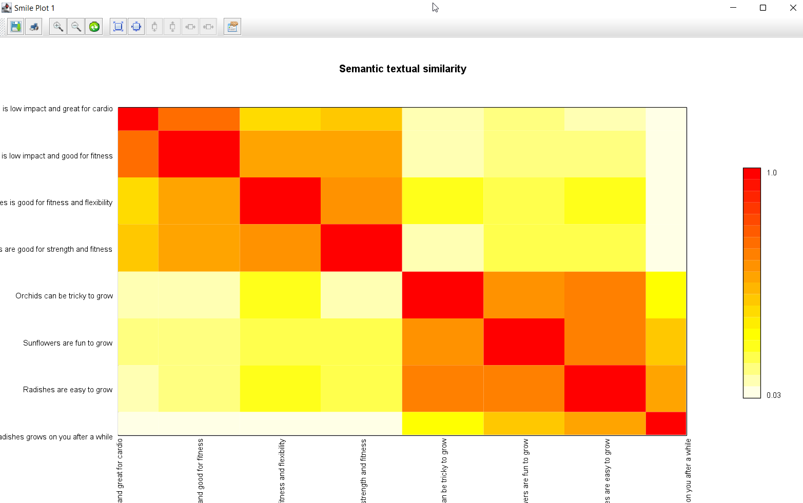
This graphic shows that our first four sentences are somewhat related, as are the last four sentences, but that there is minimal relationship between those two groups.
More information
Further examples can be found in the related repos:
Conclusion
We have look at a range of NLP examples using various NLP libraries. Hopefully you can see some cases where you could use additional NLP technologies in some of your own applications.